Variance: Order out of Chaos

In the previous post, I wrote about expectation, a great tool that helps us capture notion of “center” for a random variable. In this post, I will write about variance, another great tool that represents the “spread” of a random variable.

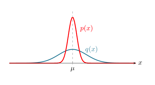
Consider a random variable $x$ with two probability density functions (PDFs) $p(x)$ and $q(x)$ , shown in the figure below. $x$ under both PDFs has the same expected value (i.e., $\mu = \E_{p(x)}[x] = \E_{q(x)}[x]$ ). But, $q(x)$ has a larger “spread” compared to $p(x)$ . In other words, samples drawn from $q(x)$ deviate more from their mean than samples drawn from $p(x)$ . Variance helps us represent this notion of spread from mean.

Definition:

The variance of a random variable $x$ is represented by $\var{x}$ and is defined by the expected value of the squared deviation from the mean $\mu = \E[x]$ :

$\var{x} = \E[(x - \mu)^2].$

$\var{x}$ is also often represented by $\sigma^2$ as the variance is the square of the standard deviation denoted by $\sigma$ .

The variance can also be expanded as:

$\begin{align*} \var{x} &= \E[(x - \mu)^2] \\ &= \E[x^2 - 2 \mu x + \mu^2 ] \\ &= \E[x^2] - 2\mu\E[x] + \mu^2 \\ &= \E[x^2] - 2\mu\mu + \mu^2 \\ &= \E[x^2] - \mu^2 \\ &= \E[x^2] - \E[x]^2. \end{align*}$

Variance is closely related to covariance that represents the linear dependency between two variables. In fact, it is easy to see that:

$\var{x} = \cov{x}{x}$

Properties:

Sign: Variance is always non-negative:

$\var{x} \geq 0.$

Shift invariance: Variance is invariant to shift:

$\var{x + c} = \var{x},$

where $c$ is a constant.

Scaling: Scaling a random variable by $c$ , scales the variance by $c^2$ :

(1) $\begin{equation*} \var{cx} = c^2\var{x}. \end{equation*}$

Sum: The variance of sum/minus is:

$\begin{align*} \var{x + y} &= \var{x} + \var{y} + 2\cov{x}{y}, \\ \var{x - y} &= \var{x} + \var{y} - 2\cov{x}{y}, \end{align*}$

where $\cov{x}{y}$ denotes the covariance between two random variables. This can be easily generalized to the sum of many random variables:

$\var{\sum_i x_i} = \sum_i \var{x_i} + 2 \sum_{i \neq j} \cov{x_i}{x_j}$

If all $x_i$ are independent or uncorrelated, we have $\cov{x_i}{x_j}=0$ , $\forall i \neq j$ . This results in:

(2) $\begin{equation*} \var{\sum_i x_i} = \sum_i \var{x_i} \end{equation*}$

Example:

Assume $x$ is a Normally-distributed random variable with mean $\mu$ and variance $\sigma^2$ , i.e., $x \sim \mathcal{N}(\mu, \sigma^2)$ . We use a Monte Carlo estimate of the mean by drawing $N$ samples from the distribution denoted by $\{x^{(n)}\}_{n=1}^{N}$ :

$\hat{\mu} = \frac{1}{N} \sum_{n=1}^{N} x^{(n)}$

what are the mean and variance of $\hat{\mu}$ ?

First, we should note that $\hat{\mu}$ itself is a random variable. In other words, it has its own distribution with its own mean and variance. Second, $\hat{\mu}$ is a stochastic estimation of $\mu$ . i.e., $\mu$ is fixed in our problem, but $\hat{\mu}$ depends on the set of samples $\{x^{(n)}\}_{n=1}^{N}$ . If we calculate $\hat{\mu}$ using a different set of samples, its value will be different.

Mean: Let’s use what we learned in the previous post to derive the mean of $\hat{\mu}$ :

$\begin{align*} \E[\hat{\mu}] &= \E[\frac{1}{N} \sum_{n=1}^{N} x^{(n)}] = \frac{1}{N} \sum_{n=1}^{N} \E[x^{(n)}] = \frac{1}{N} \sum_{n=1}^{N} \mu = \mu \end{align*}$

So, the expected value of $\hat{\mu}$ is $\mu$ .

Variance: Since the set of samples are drawn independently, we can use the sum and scaling properties (Eq.1 and 2):

$\begin{align*} \var{\hat{\mu}} &= \var{\frac{1}{N} \sum_{n=1}^{N} x^{(n)}} = \frac{1}{N^2} \var{\sum_{n=1}^{N} x^{(n)}} \\ &= \frac{1}{N^2} \sum_{n=1}^{N} \var{x^{(n)}} = \frac{N}{N^2} \var{x} = \frac{\sigma^2}{N} \end{align*}$

As you can see, the variance of $\hat{\mu}$ depends on the sample size. As the sample size grows $\var{\hat{\mu}}$ goes to zero. In fact the sum of Normally-distributed random variables has a Normal distribution itself. Thus, we have $\hat{\mu} \sim \mathcal{N}(\mu, \frac{\sigma^2}{N})$ . As $N$ increases, the distribution of $\hat{\mu}$ which is centered at $\mu$ , becomes narrower, and as a result, $\hat{\mu}$ approaches $\mu$ .

Why variance is important in training:

Recall that in the previous post I mentioned that many training objective functions take the form of an expectation. The gradient of those objective functions is also in the form of an expectation. Since in general, we don’t have an analytic expression for the expected value of the gradient, we typically use a stochastic estimation of the gradient for optimizing the objective function. In this case, the variance of the gradient estimator plays a crucial role in training. High gradient variance can extremely slow down the training progress.

In practice, many factors impact the variance of a gradient estimator. Here, we are going to analyze the effect of the training batch size. Let’s consider a model with a single parameter. We represent this model by $f_w(x)$ where $x$ is an input instance and $w$ is the parameter. For example, our model can be as simple as a linear function $f_w(x) = w x$ . Let’s denote the target variable by $y$ and the loss function measuring the mismatch between the model output $f_w(x)$ and target $y$ by $l(f_w(x), y)$ . The training objective is to find $w$ that has the lowest loss in average. This is formulated as minimizing the following expectation:

$\mathcal{L}(w) = \E_{p(x,y)}[l(f_w(x), y)],$

where $p(x,y)$ is the joint distribution of input and target variables. We can use a gradient-based optimization method to minimize $\mathcal{L}(w)$ . For this, we require computing the gradient of the loss function:

$\frac{\partial \mathcal{L}(w)}{\partial w} = \E_{p(x,y)}[\frac{\partial}{\partial w} l(f_w(x), y)]$

As you can see both the objective function $\mathcal{L}(w)$ and the gradient $\frac{\partial \mathcal{L}(w)}{\partial w}$ are in the form of an expectation.

We don’t have the joint $p(x,y)$ explicitly. Thus, we cannot compute the expectations analytically. However, the training dataset $\{(x^{(i)}, y^{(i)})\}$ are samples drawn from the joint $p(x,y)$ . We can define a Monte Carlo estimate of the gradient using a mini-batch of $M$ randomly-selected training datapoints:

$\hat{g} = \frac{1}{M}\sum_{i=1}^{M} \frac{\partial}{\partial w} l(f_w(x^{(i)}), y^{(i)}),$

where $\hat{g}$ is the stochastic estimator of $\frac{\partial \mathcal{L}(w)}{\partial w}$ . As we saw in the example, $\var{\hat{g}} = \frac{\sigma_g^2}{M}$ where $\sigma_g^2=\var{\frac{\partial}{\partial w} l(f_w(x), y)}$ . We generally don’t have $\sigma_g^2$ , so we cannot quantify $\var{\hat{g}}$ . However, it is easy to see that $\var{\hat{g}}$ reduces as the mini-batch size increases. In other words, increasing the training mini-batch size, in average, brings $\hat{g}$ closer to the true gradient.

Summary

In this post, we learned about variance and its basic properties, and we saw how we can use them to derive the mean and variance of an estimator. In the next post, we will dig deeper into an ML problem to better understand how these fundamental concepts play together during training. If you like to stay updated with the future posts, you can use the form below to subscribe.

Definition:

Properties:

Example:

Why variance is important in training:

Summary

Leave a Comment Cancel Reply