Expectations: always yours to meet

Machine learning (ML) is filled with various forms of mathematical expectations. It is not exaggerated to say that almost all training objective functions in ML are in the form of an expectation. In this blog post, I will review some basics on expectations to create a foundation for my next posts on probabilistic ML.

I personally believe that everyone should learn to use expectations for making personal decisions. Estimating the expected value of an outcome and the variance associated with it is typically used for analyzing investment opportunities by professional investors.

Simple Example:

Imagine you want to buy a lottery ticket for $2 and you would like to know what you will win on average. You know 1 million tickets are sold as part of this lottery and the prizes are:

$1M for 1 person
$10,000 for 10 people
$1,000 for 100 people
$100 for 1,000 people

Let’s look at the probability of each event:

You win $1M with probability 1 in one million $(p=10^{-6})$
You win $10K with probability 1 in 100,000 $(p=10^{-5})$
You win $1K with probability 1 in 10,000 $(p=10^{-4})$
You win $100 with probability 1 in 1,000 $(p=10^{-3})$
You win nothing with probability $(p \approx 0.999)$

Let’s represent each of these events using $x \in \mathcal{X}=\{1, 2, 3, 4, 5\}$ . We know for example $p(x=1) = 10^{-6}$ . Let’s also represent the prize you win with $f(x)$ , i.e., $f(x) =$ $1M if $x=1$ . The expected value of the prize you will win is:

$\mathbb{E}_{x\sim p(x)}[f(x)] = \sum_{x \in \mathcal{X}} p(x) f(x).$

You can think of this equation as averaging the values of an outcome with weights equal to the probability of that outcome. So, rare outcomes are weighted with smaller weights. The expected value of the prize is:

$10^{-6} \times 10^6 + 10^{-5} \times 10^4 +10^{-4} \times 10^3 + 10^{-3} \times 100 + 0 \times 0.999 = \$1.3$

So on average, you will win $1.3 by paying $2!

What amazes me here is that the number $1.3 cannot be seen easily in the list of the prizes. By looking at this list you may think that “at least you will win $100 which is 50 times what you invested ($2)”.

Definition:

If $x \in \mathcal{X}$ is a discrete random variable with $\mathcal{X}$ representing the set of all possible values of $x$ , the expected value of $f(x)$ given that $x$ has distribution $p(x)$ is denoted by:

$\mathbb{E}_{x\sim p(x)}[f(x)] = \sum_{x \in \mathcal{X}} p(x) f(x).$

Sometimes this notation is simplified to $\mathbb{E}_{p(x)}[f(x)]$ or even $\mathbb{E}[f(x)]$ if the distribution of $x$ is implied.

If $x \in \Omega$ is a continuous random variable where $\Omega$ is the sample space of $x$ , the summation is replaced by an integral:

$\mathbb{E}_{x\sim p(x)}[f(x)] = \int_\Omega p(x) f(x) dx.$

Here, $p(x)$ is the probability density function for random variable $x$ . For example if $x$ has a Normal distribution, its sample space is the space of all real numbers $\mathbb{R}$ . In this case the integral is written as:

$\mathbb{E}_{x\sim p(x)}[f(x)] = \int_{-\infty}^{+\infty} p(x) f(x) dx.$

Properties:

Let’s go over some of the properties that are commonly used in ML:

1) Mean: If $f(x) = x$ , then $\mathbb{E}_{p(x)}[f(x)]$ is the mean of the random variable $x$ .

2) Constant: If $f$ is constant, i.e., $f(x) = c$ , the expected value is also constant:

$\mathbb{E}_{p(x)}[c] = \int p(x)\,c\,dx = c\int p(x)\,dx=c.$

3) Linearity:

$\begin{align*} \mathbb{E}_{p(x)}[af(x)] &= a\mathbb{E}_{p(x)}[f(x)] \\ \mathbb{E}_{p(x, y)}[f(x)+g(y)] &= \mathbb{E}_{p(x)}[f(x)] + \mathbb{E}_{p(y)}[g(y)] \end{align*}$

where $x$ and $y$ are two random variables.

4) Jensen’s inequality: If $f(x)$ is a convex function, we have:

$f(\mathbb{E}_{p(x)}[x]) \leq \mathbb{E}_{p(x)}[f(x)]$

In other words, if you apply a convex function $f$ to the expected value of a random variable, it will be less than or equal to the expected value of the function. The direction of the inequality changes if $f$ is a concave function. I will discuss this inequality in more details in another post.

Computing an Expectation:

In many ML problems, we are often required to compute the value of an expectation. Here, I review three different approaches to tackle this problem. For this section, let’s assume we are interested in finding the expected value of a Normal random variable with mean $\mu = 3$ and standard deviation $\sigma=1$ . That is to say find:

$\mathbb{E}_{p(x)}[x] = \int_{-\infty}^{+\infty}p(x)xdx, \ \ \text{where} \ \ p(x)=\mathcal{N}(x;\mu, \sigma).$

1) Know your functions:

Solving an expectation is the same as taking the integral of a function. This function is nothing but the product of the probability density function $p(x)$ and $f(x)$ . In our example, the functions $p(x) = \mathcal{N}(x;\mu, \sigma)$ and $f(x) =x$ look like:

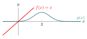
Above, it is not clear how we can take the integral of $f(x)p(x)$ . But, if $f(x)$ was shifted such that it was crossing the $x$ -axis at the mean of the Normal distribution, we would have symmetric functions. This shifted function is $x - 3$ :

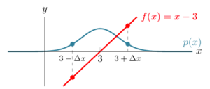
As you can see above both $p(x)$ and $f(x)=x - 3$ are symmetric around $x=3$ (the mean of the Normal distribution). The symmetry is such that if we consider two mirrored points $x_1 = 3 + \Delta x$ and $x_2 = 3 - \Delta x$ , the probability density function is equal, i.e., $p(x_1) = p(x_2)$ for any positive $\Delta x$ . But, the function $f(x)=x - 3$ is negated for those points, i.e., $f(x_1) = - f(x_2)$ . As you can guess, the product of $p(x)$ and $f(x)=x-3$ is also symmetric:

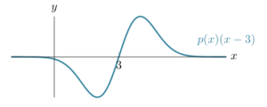
Given this symmetry, it is easy to see that the integral of $p(x)(x - 3)$ for the entire $x$ -axis is zero. This means $\mathbb{E}_{p(x)}[x - 3] = 0$ . Now, we can use this to solve our expectation problem:

$\mathbb{E}_{p(x)}[x] = \mathbb{E}_{p(x)}[x-3+3] = \mathbb{E}_{p(x)}[x-3] + \mathbb{E}_{p(x)}[3] = 0 + 3 = 3$

2) Just do the math:

So far, we have used the shape of the functions $p(x)$ and $f(x)$ to derive the expected value. In practice, visualizing a function and underlying distribution does not always result in the value of an expectation, but it gives us intuitions on how to attack the problem. Here, we will try to solve the integral directly using techniques from calculus. We have:

$\begin{align*} \mathbb{E}_{p(x)}[x] &= \mathbb{E}_{p(x)}[x - 3 + 3] = \mathbb{E}_{p(x)}[x-3] + \mathbb{E}_{p(x)}[3] \\ &= \int_{-\infty}^{+\infty}\frac{1}{\sqrt{2\pi}}e^{-\frac{(x-3)^2}{2}}(x-3)dx + 3 \end{align*}$

Note that here we use the definition of Normal distribution, i.e., $\mathcal{N}(x;3, 1)=\frac{1}{\sqrt{2\pi}}e^{-\frac{(x-3)^2}{2}}$ . Now, we can introduce the change of variable $u = \frac{(x-3)^2}{2}$ and $du = (x-3)dx$ :

$\begin{align*} \mathbb{E}_{p(x)}[x] &= \int_{+\infty}^{+\infty}\frac{1}{\sqrt{2\pi}}e^{-u}du + 3 \\ &= - \frac{1}{\sqrt{2\pi}} e^{-u} \big]_{+\infty}^{+\infty} + 3 = 0 + 3 = 3 \end{align*}$

3) Draw Samples:

The most general approach for solving an expectation is to use a sampling-based method called the Monte Carlo method. This approach can be used only if we can draw samples from distribution $p(x)$ . Let’s represent a set of $L$ samples from $p(x)$ by $\{x^{(1)}, x^{(2)}, \dots, x^{(L)}\}$ . Based on the Monte Carlo method, we have:

$\mathbb{E}_{p(x)}[x] \approx \frac{1}{L} \sum_{l=1}^{L} x^{(l)},$

which is to say that the expected value is approximated by taking the average of samples drawn from the distribution. For example, let’s draw 10 samples from $p(x) = \mathcal{N}(x;3, 1)$ :

$\{2.71, 4.45, 4.20, 3.12, 2.73, 1.17, 3.08, 0.56, 2.82, 2.94 \}$

If we take the average of these 10 samples, we will have $\mathbb{E}_{p(x)}[x] \approx 2.78.$ Note that this estimate is not exactly the same as the estimate we get with the previous approaches. This is because the Monte Carlo method provides a stochastic estimation of the integral. This estimation is unbiased meaning that on average it is always equal to the true value. However, it contains variance (i.e., deviation from the true value). We will discuss this in more details later.

Summary

In this post, I reviewed some basic properties of expectations and a few simple techniques for computing them. Among these techniques, the Monte Carlo method is widely used in ML especially if there is no closed-form derivation for an expectation. However, I typically find visualizing functions and distributions very informative, although it may not yield to a solution directly.

As you may know, I am just about to start this blog, and I need your help to reach out to a greater audience. So, if you like this post, please don’t hesitate to share it with your network. If you have any suggestion, please post it in the comments section.

5 thoughts on “Expectations: always yours to meet”

Maysam
14th December 2018 at 7:43 am

I like the clarity and pace of your writing. Tnx
Keep it up please

1. Arash
  16th December 2018 at 8:46 pm
  
  Thank you!
  
Oren
14th December 2018 at 4:59 pm

Very clear explanation, please keep it up!

Jae Duk Seo
15th December 2018 at 10:13 am

very good blog post

Nasser
2nd January 2019 at 4:51 pm

Thanks for sharing this. Very easy to follow and well written. I am looking forward for the next post.